In the previous post, we took the data that we exported from Google Maps Timeline processed it and uploaded it to Google BigQuery for analysis.

Today we are going to do an exploratory data analysis of the information.

The example above is an example of the JSON information that we get from Google. I should mention that I’m not an expert in GPS information, so I’ve tried to do some research on all of this. If you find something wrong, you can open a pull request and help me fix it.

As you can see from the file above we have a lot of rich metadata here that we can use.

Value	Meaning
heading	The direction the device is traveling.
activity.type	Here, activity could refer to multiple values. My guess is that Google is using some machine learning magic to infer what the user is potentially doing. There are many possible values.
activity.confidence	Here, Google is assigning a confidence interval to your activity type. The values go from low to high, 0 - 100.
activity.timestampMs	This is the timestamp in milliseconds for the recorded activity.
verticalAccuracy	This could refer to the accuracy of the vertical location of the device.
velocity	This could refer to the speed of the device at capture time. It’s probably inferred based on other data points.
accuracy	Accuracy is Google’s estimate of how accurate the data is. An accuracy of less than 800 is high and more than 5000 is low.
longitudeE7	This is the longitudinal value of the observation.
latitudeE7	This is the latitudinal value of the observation.
altitude	This could refer to the altitude of the device. I’m assuming it’s measured from sea level.
timestampMs	This is the timestamp in milliseconds that the observation was recorded.

For the main values that we’ll be working with: timestampMs, longitudeE7 and latitudeE7. These values are not in great “human readable” format, but BigQuery can help us fix that!

In BigQuery, we can convert this timestampMs 1486800415000 to 2017-02-11 08:06:55.000 UTC using MSEC_TO_TIMESTAMP().

We can also easily convert latitudeE7 and longitudeE7 by dividing by 1e7. 481265044/1e7 becomes 48.1265044 and 116593258/1e7 is 11.6593258 giving us the coordinates 48.1265044, 11.6593258 which is 48°07'35.4"N 11°39'33.6"E.

If you want to read more about latitude and longitude, check out Understanding Latitude and Longitude.

Also in the example data above looking at the activity for this observation Google thinks it’s 75% confident that I’m in a vehicle going somewhere.

Exploratory Data Analysis

Now that we have looked at the data available in the JSON file, let’s write some SQL and pull all of the information into R and take a look at what’s going on.

For this analysis, I’ll be analyzing the following:

values	type	definition
latitude	FLOAT	The latitude of the observation
longitude	FLOAT	The longitude of the observation
date	TIMESTAMP	The date, converted from timestampMs
accuracy	INTEGER	The accuracy of the observation
accuracyLevel	STRING	The inferred accuracy level of the observation
minuteDifference	FLOAT	The difference in minutes between current and previous observation
activityType	STRING	The type of activity of the observation
activityConfidence	INTEGER	The confidence level of the activity
latLong	STRING	The concatenated values of Latitude and Longitude
cityLatLong	STRING	Values of the lat/lon used to guess the current city

The table above is generated by running the Legacy SQL code below in BigQuery.

There are a few ways you can handle this. In my R code, I’ve written the query to pull the results directly into a local data frame. You can also run the query and save the results to a temp table, to help reduce calls and save yourself a little bit of money. It’s personal preference.

Overall

Let’s begin our analysis by looking at some simple questions:

1. How many observations do we have? We have 1,770,882 recorded observations.
2. What is the minimum recorded time? 2011-07-24 03:59:37 UTC
3. What is the maximum recorded time? 2018-03-21 11:46:00 UTC
4. What is the median time difference between observations? 60 seconds
5. How many different coordinates were recorded? 418,890

Wow, so ~1.7mil observations between 2011 and 2018. That’s a lot considering that observations are sent every 60 seconds! There are 10,081 observations recorded 26 seconds apart. That might be worth investigating more.

Another thing that I’ve observed is that since observations depend on cell towers, satellites and WIFI they can sometimes be inaccurate even when you’re standing still.

Take for example these two locations: 40.555653, -105.098351 and 40.555608, -105.098397.

Even though my phone may be sitting quietly in a locker sometimes the distance recorded between observations may be 20 feet apart. It’s hard to tell without visualizing it, so I’m not going to worry about that for now.

Accuracy

How accurate are the observations? 95% of all observations are rated as HIGH with less than 0.01% with an accuray of LOW.

accuracyLevel	n
high	1696926
medium	73637
low	319

Activities

activityType	count	medianConfidence
still	549051	100
tilting	65220	100
unknown	35531	75
in vehicle	33277	85
on foot	15554	80
exiting vehicle	964	100
on bicycle	866	75

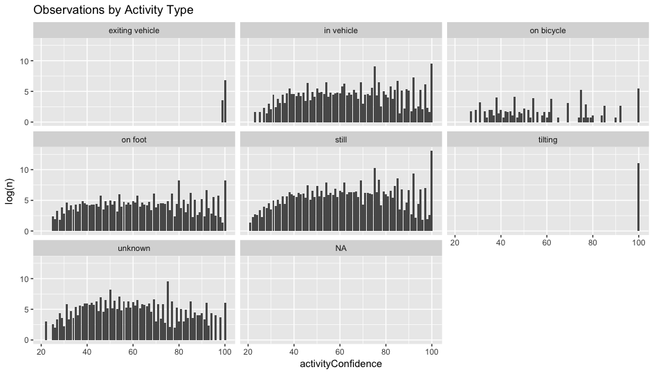
As you can see, we seven different types of activity, excluding NA’s. It would be interesting to try to figure out what’s going on with the unknown and NA.

Lets visualize the distribution by activity type. All of the observations are left skewed so we are going to visualize this using log.

Here’s the R code if you would like to follow along: