In part one we walked through the steps of getting set up to pull data from Google Adwords using the RAdwords package. Today we’ll dive in a bit deeper with some exploratory data analysis.
Let’s get started shall we?
yesterday <- gsub("-","",format(Sys.Date()-1,"%Y-%m-%d"))
thirtydays<- gsub("-","",format(Sys.Date()-29,"%Y-%m-%d"))

# Create statement
body <- statement(select = c(
  "CampaignName",
  "AdGroupName",
  "Criteria",
  "KeywordMatchType",
  "QualityScore",
  "Impressions",
  "Clicks",
  "Ctr",
  "ConvertedClicks",
  "AverageCpc",
  "Cost",
  "Date"),
  report = "KEYWORDS_PERFORMANCE_REPORT",
  where = "AdNetworkType1 = SEARCH",
  start = thirtydays,

# Pull data from Adwords
data <- getData(clientCustomerId='xxx-xxx-xxxx', google_auth=google_auth, statement=body)
First lets walk through what’s happening with the code. The first two variables yesterday and thirtydays will take the current system date and format it for Adwords. It will give us the dates from 30 days ago and yesterday’s date.
Second, the variable body constructs our satement that we’ll use to request Adwords data. Here we’re asking for Keywords Performance Report data for Search Networks for the past thirty days. We’ll get the following items in return:
- Campaign Name
- Ad Group Name
- Criteria (Keyword)
- Keyword Match Type (Broad, Phrase, Exact)
- Quality Score
- Impressions
- Clicks
- Click Through Rate (Clicks divided by Impressions)
- Conversions
- Average Cost Per Click (Clicks divided by Cost)
- Cost
- Date
Here the date variable, although last is still important. When we call the AdWords API, we’ll get all of the results for each day in the call. That’s great!
Third, we are going to save the call with getData() to a data frame called data. Once the results have been returned, we can begin our analysis.
Quality Score
To begin with, let’s run summary(data). This will gives us a summary of our data frame. One of the most important factors with keywords are the Quality Score of your keywords. The higher your Quality Score, the lower your CPC.
Let’s breakout the performance using dplyr, grouping by Quality Score and counting keywords:
data %>%
group_by(Qualityscore) %>%
summarize(keywords = length(Keyword))
| Qualityscore | keywords |
|---|---|
| 10 | 1 |
| 2 | 2 |
| 3 | 6 |
| 4 | 4 |
| 5 | 9 |
| 6 | 3 |
| 7 | 9 |
| 8 | 8 |
| 9 | 7 |
Let’s also plot a histogram to visualize the same information:
data %>%
  ggplot(aes(Qualityscore)) +
  geom_histogram(bins = 20) +
  labs(title = "Histogram of Quality Score",
       x = "Quality Score",
       y = "Count")
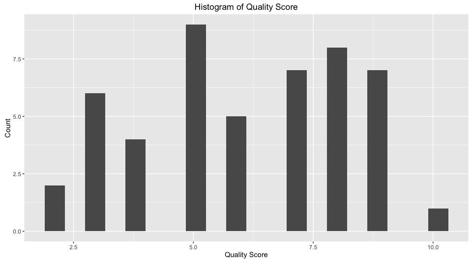
We can see that there are 21 keywords with a Quality Score lower than six. Depending on the goals and needs of your campaigns, you may want to save these for later to pause or rewrite the ads associated with the keywords. You can do that using:
keywordsToChange <- data %>%
filter(Qualityscore < 6)
The quickest win that you get with your account is to increase the quality score. There are at least three main factors that affect your quality score:
- Expected Click-Through Rate
- Ad Relevance
- Landing Page Experience
You can also add the following variables to your body request if you’d like to see them: SearchPredictedCtr, CreativeQualityScore and PostClickQualityScore.
Linear Regression
One of the quickest assumptions that people make about Adwords is that increasing your spend or your cost per click will automatically increase the number of conversions that you’ll recieve for that keyword.
To test that assumption, let’s build a linear regression model which can be done with lm(data$Conversions ~ data$CPC) and we can look at the full summary with summary(lm(data$Conversions ~ data$CPC))
##
## Call:
## lm(formula = data$Conversions ~ data$CPC)
##
## Residuals:
##      Min       1Q   Median       3Q      Max
## -0.13118 -0.13118 -0.08722 -0.01500  1.87878
##
## Coefficients:
##             Estimate Std. Error t value Pr(>|t|)
## (Intercept)  0.13118    0.06668   1.967   0.0551 .
## data$CPC    -0.03499    0.03193  -1.096   0.2787
## ---
## Signif. codes:  0 '***' 0.001 '**' 0.01 '*' 0.05 '.' 0.1 ' ' 1
##
## Residual standard error: 0.3431 on 47 degrees of freedom
## Multiple R-squared:  0.02492,	Adjusted R-squared:  0.00417
## F-statistic: 1.201 on 1 and 47 DF,  p-value: 0.2787
Our toy model here only explains 0.417% of the variation, so we may want to go back and look more at the outliers and build another model.
With an r-squared of 0.00417 we would want to visualize our data to visualize our assumptions.
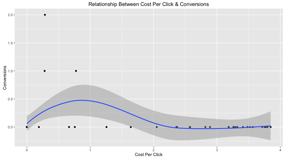
Once our linear regression model has been fixed, we can build a way to predict how many conversions we would get if we raised or lowered the cost per click.
In the next post, we’ll look at more ways of working with Adwords data.